library(pacman)
p_load(tidyverse)Network Science
Chapter 20: Network Science
This is some of the code from Chapter 20. I was able to get the PageRank code to work.
library(mdsr)
library(igraph)
Attaching package: 'igraph'The following objects are masked from 'package:lubridate':
%--%, unionThe following objects are masked from 'package:dplyr':
as_data_frame, groups, unionThe following objects are masked from 'package:purrr':
compose, simplifyThe following object is masked from 'package:tidyr':
crossingThe following object is masked from 'package:tibble':
as_data_frameThe following objects are masked from 'package:stats':
decompose, spectrumThe following object is masked from 'package:fs':
pathThe following object is masked from 'package:base':
unionn <- 100
p_star <- log(n)/n
plot_er <- function(n, p, ...) {
g <- erdos.renyi.game(n, p)
plot(g, main = paste("p =", round(p, 4)), vertex.frame.color = "white", vertex.size = 3, vertex.label = NA, ...)
}
plot_er(n, p = 0.8 * p_star)
plot_er(n, p = 1.2 * p_star)
n <- 1000
p_star <- log(n)/n
ps <- rep(seq(from = 0, to = 2 * p_star, by = 0.001), each = 100)
er_connected <- function(n, p, ...) {
  c(n = n, p = p, connected = is.connected(erdos.renyi.game(n, p)))
}
sims <- as.data.frame(t(sapply(ps, er_connected, n = n)))

ggplot(data = sims, aes(x = p, y = connected)) +
  geom_vline(xintercept = p_star, color = "darkgray") +
  geom_text(x = p_star, y = 0.9, label = "Threshold value", hjust="right") + labs(x = "Probability of edge existing",
                                                                                  y = "Probability that random graph is
                                                                                  connected") + geom_count() +
  geom_smooth()
`geom_smooth()` using method = 'gam' and formula = 'y ~ s(x, bs = "cs")'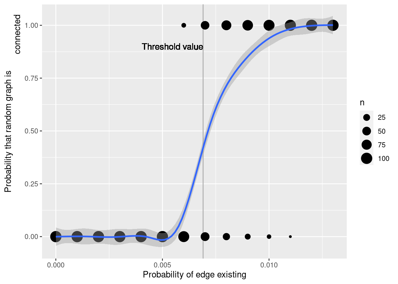
g1 <- erdos.renyi.game(n, p = log(n)/n)
g2 <- barabasi.game(n, m = 3, directed = FALSE)

summary(g1)
IGRAPH 083eeb1 U--- 1000 3557 -- Erdos-Renyi (gnp) graph
+ attr: name (g/c), type (g/c), loops (g/l), p (g/n)summary(g2)IGRAPH cab8ec5 U--- 1000 2994 -- Barabasi graph
+ attr: name (g/c), power (g/n), m (g/n), zero.appeal (g/n), algorithm
| (g/c)d <- data.frame(type = rep(c("Erdos-Renyi", "Barabasi-Albert"), each = n), degree = c(degree(g1), degree(g2)))
ggplot(data = d, aes(x = degree, color = type)) +
geom_density(size = 2) +
scale_x_continuous(limits = c(0, 25))Warning: Using `size` aesthetic for lines was deprecated in ggplot2 3.4.0.
ℹ Please use `linewidth` instead.Warning: Removed 16 rows containing non-finite values (`stat_density()`).
Extended example: 1996 men’s college backetball
To get the example to run I downloaded the data from the kaggle website for the March Machine Learning Mania 2015. You need to have an account and your needs to log in to download the data. Note that the data file that is needed to run the example has a different name than the name in the book.
library(mdsr)
teams <- readr::read_csv("data/all/teams.csv")
Rows: 364 Columns: 2
── Column specification ────────────────────────────────────────────────────────
Delimiter: ","
chr (1): team_name
dbl (1): team_id
ℹ Use `spec()` to retrieve the full column specification for this data.
ℹ Specify the column types or set `show_col_types = FALSE` to quiet this message.games <- readr::read_csv("data/all/regular_season_compact_results.csv") %>%
filter(season == 1996) Rows: 134566 Columns: 8
── Column specification ────────────────────────────────────────────────────────
Delimiter: ","
chr (1): wloc
dbl (7): season, daynum, wteam, wscore, lteam, lscore, numot
ℹ Use `spec()` to retrieve the full column specification for this data.
ℹ Specify the column types or set `show_col_types = FALSE` to quiet this message.dim(games)[1] 4122 8E <- games %>%
mutate(score_ratio = wscore/lscore) %>%
select(lteam, wteam, score_ratio)
V <- teams %>%
filter(team_id %in% unique(c(E$lteam, E$wteam)))
library(igraph)
g <- graph_from_data_frame(E, directed = TRUE, vertices = V)
summary(g)IGRAPH 2d3e1c2 DN-- 305 4122 --
+ attr: name (v/c), team_name (v/c), score_ratio (e/n)g <- set_vertex_attr(g, "pagerank", value = page_rank(g)$vector)
as_data_frame(g, what = "vertices") %>%
arrange(desc(pagerank)) %>%
head(20) name team_name pagerank
1203 1203 G Washington 0.021863566
1269 1269 Massachusetts 0.020504852
1207 1207 Georgetown 0.016415082
1234 1234 Iowa 0.014343587
1163 1163 Connecticut 0.014084209
1437 1437 Villanova 0.013089525
1246 1246 Kentucky 0.012735610
1345 1345 Purdue 0.011456116
1280 1280 Mississippi St 0.011368140
1210 1210 Georgia Tech 0.010578926
1112 1112 Arizona 0.010255324
1448 1448 Wake Forest 0.010081101
1242 1242 Kansas 0.009917330
1336 1336 Penn St 0.009752762
1185 1185 E Michigan 0.009707138
1393 1393 Syracuse 0.009563255
1266 1266 Marquette 0.009441184
1314 1314 North Carolina 0.009415234
1153 1153 Cincinnati 0.009396704
1396 1396 Temple 0.008595410wins <- E %>%
group_by(wteam) %>%
summarise(N = n())
losses <- E %>%
group_by(lteam) %>%
summarise(N = n())
wins %>% full_join(losses, by = c("wteam" = "lteam")) %>%
left_join(teams, by = c("wteam" = "team_id")) %>%
rename(wins = N.x, losses = N.y) %>%
mutate(win_pct = wins / (wins + losses)) %>%
arrange(desc(win_pct)) %>%
head(20)# A tibble: 20 × 5
wteam wins losses team_name win_pct
<dbl> <int> <int> <chr> <dbl>
1 1269 31 1 Massachusetts 0.969
2 1403 28 1 Texas Tech 0.966
3 1163 30 2 Connecticut 0.938
4 1246 28 2 Kentucky 0.933
5 1180 25 3 Drexel 0.893
6 1453 24 3 WI Green Bay 0.889
7 1158 22 3 Col Charleston 0.88
8 1307 26 4 New Mexico 0.867
9 1153 25 4 Cincinnati 0.862
10 1242 25 4 Kansas 0.862
11 1172 22 4 Davidson 0.846
12 1345 25 5 Purdue 0.833
13 1448 23 5 Wake Forest 0.821
14 1185 22 5 E Michigan 0.815
15 1439 22 5 Virginia Tech 0.815
16 1437 25 6 Villanova 0.806
17 1112 24 6 Arizona 0.8
18 1428 23 6 Utah 0.793
19 1265 22 6 Marist 0.786
20 1114 21 6 Ark Little Rock 0.778E %>% filter(wteam == 1269 & lteam == 1246)# A tibble: 1 × 3
lteam wteam score_ratio
<dbl> <dbl> <dbl>
1 1246 1269 1.12E %>% filter(lteam %in% c(1203, 1269) & wteam %in% c(1203, 1269))# A tibble: 2 × 3
lteam wteam score_ratio
<dbl> <dbl> <dbl>
1 1269 1203 1.13
2 1203 1269 1.14A_10 <- c("Massachusetts", "Temple", "G Washington", "Rhode Island", "St Bonaventure", "St Joseph's PA", "Virginia Tech", "Xavier", "Dayton", "Duquesne", "La Salle", "Fordhham")a10 <- V(g)[ team_name %in% A_10 ]
a <- induced_subgraph(g, vids = a10)
a <- set_vertex_attr(a, "pagerank", value = page_rank(a)$vector)
summary(a)IGRAPH 03a9a19 DN-- 11 90 --
+ attr: name (v/c), team_name (v/c), pagerank (v/n), score_ratio (e/n)library(ggnetwork)
library(intergraph)
a_df <- ggnetwork(a) Warning in format_fortify(model = model, nodes = nodes, weights = "none", :
duplicated edges detectedggplot(a_df, aes(x, y, xend = xend, yend = yend)) +
geom_edges(aes(alpha = score_ratio), color = "lightgray", arrow = arrow(length = unit(0.2, "cm")), curvature = 0.2) +
geom_nodes(aes(size = pagerank, color = pagerank), alpha = 0.6) + geom_nodetext(aes(label = team_name)) +
scale_alpha_continuous(range = c(0.4, 1)) +
scale_size_continuous(range = c(1, 10)) +
guides(color = guide_legend("PageRank"), size=guide_legend("PageRank")) +
theme_blank()
P <- t(as_adjacency_matrix(a, sparse = FALSE, attr = "score_ratio"))
P <- scale(P, center = FALSE, scale = colSums(P))
round(P, 2)
1173 1182 1203 1247 1269 1348 1382 1386 1396 1439 1462
1173 0.00 0.09 0.00 0.10 0 0.14 0.11 0.00 0.00 0.00 0.16
1182 0.11 0.00 0.00 0.11 0 0.00 0.00 0.00 0.00 0.00 0.00
1203 0.14 0.12 0.00 0.10 1 0.14 0.11 0.17 0.33 0.27 0.16
1247 0.00 0.09 0.25 0.00 0 0.00 0.12 0.00 0.00 0.00 0.00
1269 0.14 0.09 0.26 0.12 0 0.14 0.12 0.16 0.41 0.25 0.15
1348 0.00 0.10 0.00 0.11 0 0.00 0.13 0.16 0.26 0.21 0.18
1382 0.13 0.08 0.00 0.00 0 0.14 0.00 0.00 0.00 0.00 0.00
1386 0.13 0.09 0.24 0.10 0 0.14 0.10 0.00 0.00 0.00 0.00
1396 0.14 0.15 0.00 0.13 0 0.15 0.10 0.16 0.00 0.27 0.19
1439 0.11 0.10 0.25 0.12 0 0.14 0.11 0.17 0.00 0.00 0.15
1462 0.11 0.09 0.00 0.11 0 0.00 0.12 0.18 0.00 0.00 0.00
attr(,"scaled:scale")
1173 1182 1203 1247 1269 1348 1382 1386
9.580291 12.193997 4.385632 10.705995 1.131579 7.620903 10.466131 6.573151
1396 1439 1462
4.110908 5.112315 6.894009 v0 <- rep(1, vcount(a)) / vcount(a)
v0 [1] 0.09090909 0.09090909 0.09090909 0.09090909 0.09090909 0.09090909
[7] 0.09090909 0.09090909 0.09090909 0.09090909 0.09090909v <- v0
for (i in 1:20) {
v <- P %*% v
}
as.vector(v) [1] 0.02620462 0.01073061 0.28880610 0.07414360 0.18416968 0.07731754
[7] 0.01477331 0.09291498 0.08133820 0.11927412 0.03032723page_rank(a)$vect 1173 1182 1203 1247 1269 1348 1382
0.03683789 0.02134844 0.25160534 0.07006017 0.18793707 0.07779895 0.02541142
1386 1396 1439 1462
0.08807760 0.09042641 0.11095533 0.03954137 page_rank(a, damping = 1)$vecWarning in page_rank(a, damping = 1): At core/centrality/prpack.cpp:82 :
Damping factor is 1. Damping values close to 1 may lead to numerical
instability when using PRPACK. 1173 1182 1203 1247 1269 1348
0.023832141 0.008035839 0.288239781 0.073484127 0.204591471 0.072857810
1382 1386 1396 1439 1462
0.011052515 0.091039461 0.084180455 0.115619832 0.027066568 w <- v0
d <- 0.85
for (i in 1:20) {
w <- d * P %*% w + (1 - d) * v0
}
as.vector(w) [1] 0.04033680 0.02382045 0.25181394 0.07127669 0.16836965 0.08332106
[7] 0.02933482 0.08934652 0.08765190 0.11231744 0.04241073page_rank(a, damping = 0.85)$vector 1173 1182 1203 1247 1269 1348 1382
0.03683789 0.02134844 0.25160534 0.07006017 0.18793707 0.07779895 0.02541142
1386 1396 1439 1462
0.08807760 0.09042641 0.11095533 0.03954137