statebins

This notebook introduces the ideas of statebins.

This is for working on the Project. Find some economic data from the FRED website. For example take the data from a map and make a statebin from it.

Use the socviz Chapter 7 Section 3 as a reference.

From the Preface of the book load the following packages, install and load the socviz and statebin package from the authors github.

library(pacman)
p_load("tidyverse", "broom", "coefplot", "cowplot",
                 "gapminder", "GGally", "ggrepel", "ggridges", "gridExtra",
                 "here", "interplot", "margins", "maps", "mapproj",
                 "mapdata", "MASS", "quantreg", "rlang", "scales",
                 "survey", "srvyr", "viridis", "viridisLite", "devtools", "socviz", "statebins")

Installing package into '/home/esuess/R/x86_64-pc-linux-gnu-library'
(as 'lib' is unspecified)

also installing the dependency 'useful'

coefplot installed

Installing package into '/home/esuess/R/x86_64-pc-linux-gnu-library'
(as 'lib' is unspecified)

also installing the dependencies 'broom.helpers', 'ggstats'

GGally installed

Installing package into '/home/esuess/R/x86_64-pc-linux-gnu-library'
(as 'lib' is unspecified)

also installing the dependencies 'arm', 'interactionTest'

interplot installed

Installing package into '/home/esuess/R/x86_64-pc-linux-gnu-library'
(as 'lib' is unspecified)

also installing the dependency 'prediction'

margins installed

Installing package into '/home/esuess/R/x86_64-pc-linux-gnu-library'
(as 'lib' is unspecified)

mapdata installed

Installing package into '/home/esuess/R/x86_64-pc-linux-gnu-library'
(as 'lib' is unspecified)

also installing the dependency 'mitools'

survey installed

Installing package into '/home/esuess/R/x86_64-pc-linux-gnu-library'
(as 'lib' is unspecified)

srvyr installed

Installing package into '/home/esuess/R/x86_64-pc-linux-gnu-library'
(as 'lib' is unspecified)

socviz installed

data("election")

election %>% select(state, total_vote,
                    r_points, pct_trump, party, census) %>%
    sample_n(5)

# A tibble: 5 × 6
  state                total_vote r_points pct_trump party      census   
  <chr>                     <dbl>    <dbl>     <dbl> <chr>      <chr>    
1 Oregon                  2001336   -11.0      39.1  Democratic West     
2 Massachusetts           3325046   -27.2      32.8  Democratic Northeast
3 Florida                 9502747     1.19     48.6  Republican South    
4 District of Columbia     311268   -86.8       4.09 Democratic South    
5 Idaho                    690433    31.8      59.2  Republican West     

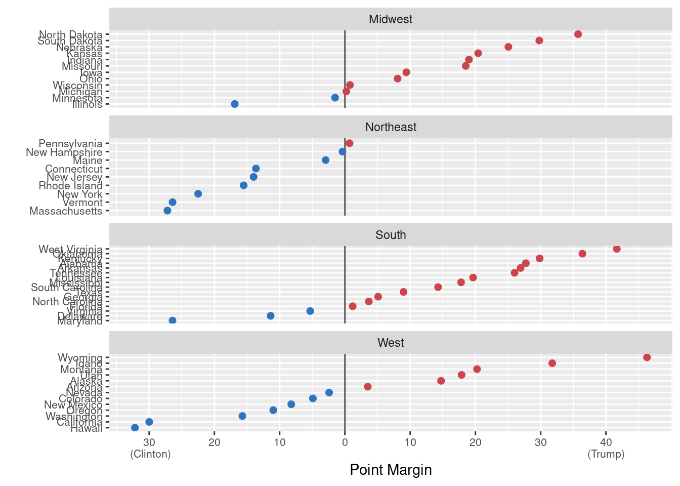
# Hex color codes for Dem Blue and Rep Red
party_colors <- c("#2E74C0", "#CB454A") 

p0 <- ggplot(data = subset(election, st %nin% "DC"),
             mapping = aes(x = r_points,
                           y = reorder(state, r_points),
                           color = party))

p1 <- p0 + geom_vline(xintercept = 0, color = "gray30") +
    geom_point(size = 2)

p2 <- p1 + scale_color_manual(values = party_colors)

p3 <- p2 + scale_x_continuous(breaks = c(-30, -20, -10, 0, 10, 20, 30, 40),
                              labels = c("30\n (Clinton)", "20", "10", "0",
                                         "10", "20", "30", "40\n(Trump)"))

p3 + facet_wrap(~ census, ncol=1, scales="free_y") +
    guides(color=FALSE) + labs(x = "Point Margin", y = "") +
    theme(axis.text=element_text(size=8))

Warning: The `<scale>` argument of `guides()` cannot be `FALSE`. Use "none" instead as
of ggplot2 3.3.4.

library(maps)
us_states <- map_data("state")
head(us_states)

       long      lat group order  region subregion
1 -87.46201 30.38968     1     1 alabama      <NA>
2 -87.48493 30.37249     1     2 alabama      <NA>
3 -87.52503 30.37249     1     3 alabama      <NA>
4 -87.53076 30.33239     1     4 alabama      <NA>
5 -87.57087 30.32665     1     5 alabama      <NA>
6 -87.58806 30.32665     1     6 alabama      <NA>

dim(us_states)

[1] 15537     6

p <- ggplot(data = us_states,
            mapping = aes(x = long, y = lat,
                          group = group))

p + geom_polygon(fill = "white", color = "black")

p <- ggplot(data = us_states,
            aes(x = long, y = lat,
                group = group, fill = region))

p + geom_polygon(color = "gray90", size = 0.1) + guides(fill = FALSE)

Warning: Using `size` aesthetic for lines was deprecated in ggplot2 3.4.0.
ℹ Please use `linewidth` instead.

p <- ggplot(data = us_states,
            mapping = aes(x = long, y = lat,
                          group = group, fill = region))

p + geom_polygon(color = "gray90", size = 0.1) +
    coord_map(projection = "albers", lat0 = 39, lat1 = 45) +
    guides(fill = "none")

election$region <- tolower(election$state)
us_states_elec <- left_join(us_states, election)

Joining with `by = join_by(region)`

p <- ggplot(data = us_states_elec,
            aes(x = long, y = lat,
                group = group, fill = party))

p + geom_polygon(color = "gray90", size = 0.1) +
    coord_map(projection = "albers", lat0 = 39, lat1 = 45) 

p0 <- ggplot(data = us_states_elec,
             mapping = aes(x = long, y = lat,
                           group = group, fill = party))
p1 <- p0 + geom_polygon(color = "gray90", size = 0.1) +
    coord_map(projection = "albers", lat0 = 39, lat1 = 45) 
p2 <- p1 + scale_fill_manual(values = party_colors) +
    labs(title = "Election Results 2016", fill = NULL)
p2 + theme_map() 

Trump vote default colors not so good.

p0 <- ggplot(data = us_states_elec,
             mapping = aes(x = long, y = lat, group = group, fill = pct_trump))

p1 <- p0 + geom_polygon(color = "gray90", size = 0.1) +
    coord_map(projection = "albers", lat0 = 39, lat1 = 45) 

p1 + labs(title = "Trump vote") + theme_map() + labs(fill = "Percent")

p2 <- p1 + scale_fill_gradient(low = "white", high = "#CB454A") +
        labs(title = "Trump vote") 
p2 + theme_map() + labs(fill = "Percent")

Winning percentage, again default colors are not so good.

p0 <- ggplot(data = us_states_elec,
             mapping = aes(x = long, y = lat, group = group, fill = d_points))

p1 <- p0 + geom_polygon(color = "gray90", size = 0.1) +
    coord_map(projection = "albers", lat0 = 39, lat1 = 45) 

p2 <- p1 + scale_fill_gradient2() + labs(title = "Winning margins") 
p2 + theme_map() + labs(fill = "Percent")

p3 <- p1 + scale_fill_gradient2(low = "red", mid = scales::muted("purple"),
                                high = "blue", breaks = c(-25, 0, 25, 50, 75)) +
    labs(title = "Winning margins") 
p3 + theme_map() + labs(fill = "Percent")

Without Washington Dc

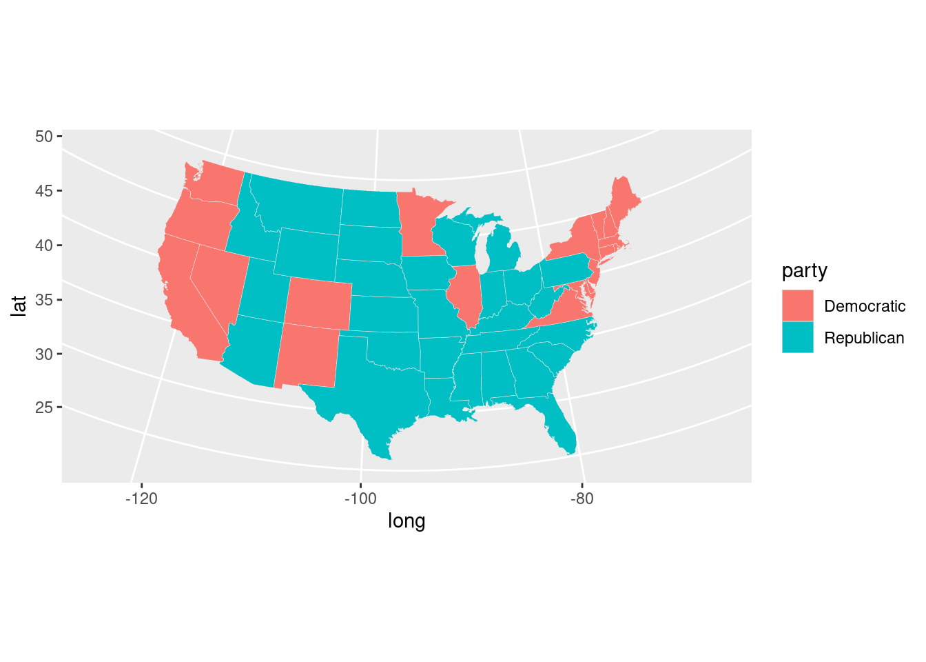
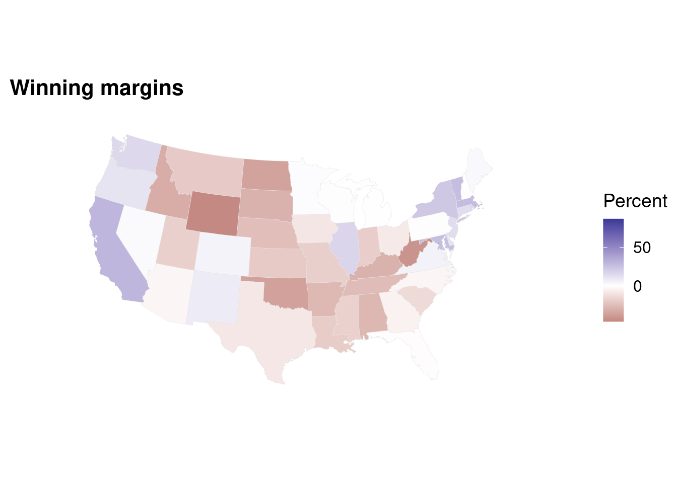
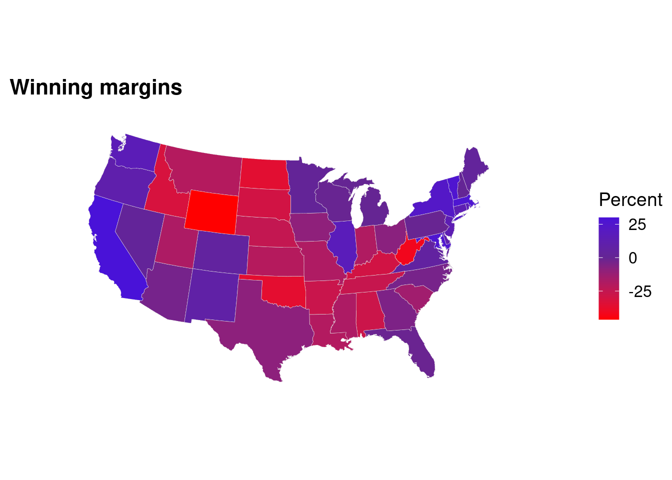
p0 <- ggplot(data = subset(us_states_elec,
                           region %nin% "district of columbia"),
             aes(x = long, y = lat, group = group, fill = d_points))

p1 <- p0 + geom_polygon(color = "gray90", size = 0.1) +
    coord_map(projection = "albers", lat0 = 39, lat1 = 45) 

p2 <- p1 + scale_fill_gradient2(low = "red",
                                mid = scales::muted("purple"),
                                high = "blue") +
    labs(title = "Winning margins") 
p2 + theme_map() + labs(fill = "Percent")

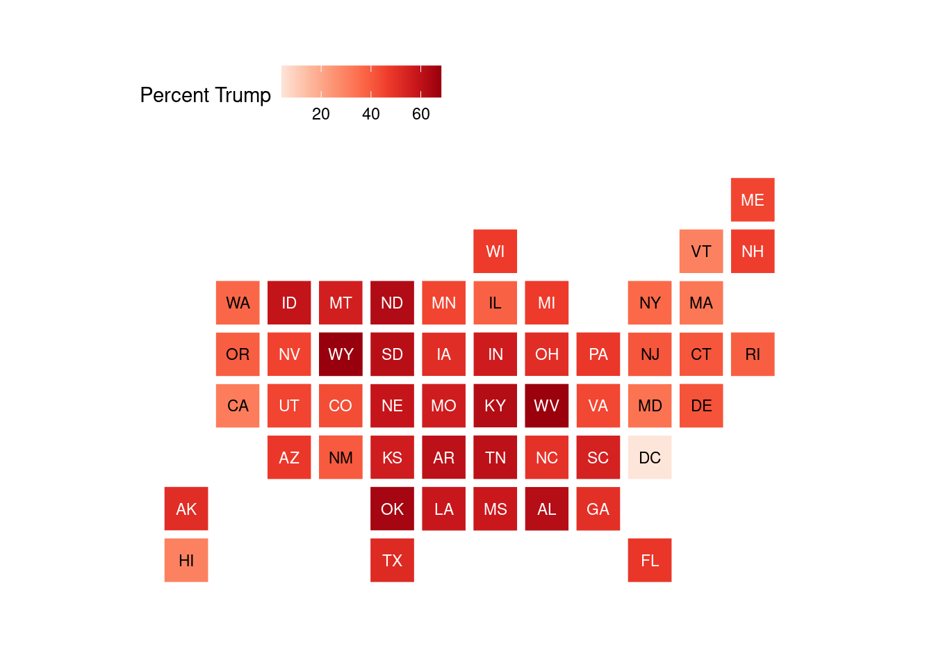
Statebins Fix this using ggplot() and geom_statebins()

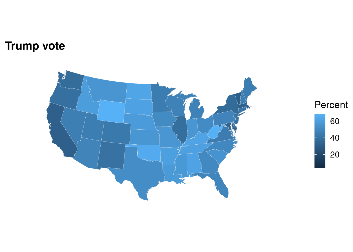
library(statebins)

election %>% statebins(value_col = "pct_trump", name = "Percent Trump",
                       palette = "Reds", direction = 1) +
  theme_statebins(legend_position="top")

state_data <- filter(election, st %in% "DC")
state_data

# A tibble: 1 × 23
  state      st     fips total_vote vote_margin winner party pct_margin r_points
  <chr>      <chr> <dbl>      <dbl>       <dbl> <chr>  <chr>      <dbl>    <dbl>
1 District … DC       11     311268      270107 Clint… Demo…      0.868    -86.8
# ℹ 14 more variables: d_points <dbl>, pct_clinton <dbl>, pct_trump <dbl>,
#   pct_johnson <dbl>, pct_other <dbl>, clinton_vote <dbl>, trump_vote <dbl>,
#   johnson_vote <dbl>, other_vote <dbl>, ev_dem <dbl>, ev_rep <dbl>,
#   ev_oth <dbl>, census <chr>, region <chr>

election %>% statebins(value_col = "pct_clinton", name = "Percent Clinton",
                       palette = "Blues", direction = 1) +
  theme_statebins(legend_position="top")