Chloropleth maps and Heatmaps
Today we will discuss the use of choropleth maps and heatmaps.
Choropleth maps add color to states relative to a variable.
Heatmaps visual the values in a matrix by add color relative to a variable(s), usually down columns.
Choropleth maps
The R packages choroplethr and choroplethrMaps can be used to make choropleth maps.
To learn about this package consider taking the free course
Choropleth maps
library(tidyverse)
library(choroplethr)
library(choroplethrMaps)

data(df_pop_state)
head(df_pop_state, 15)
                 region    value
1               alabama  4777326
2                alaska   711139
3               arizona  6410979
4              arkansas  2916372
5            california 37325068
6              colorado  5042853
7           connecticut  3572213
8              delaware   900131
9  district of columbia   605759
10              florida 18885152
11              georgia  9714569
12               hawaii  1362730
13                idaho  1567803
14             illinois 12823860
15              indiana  6485530
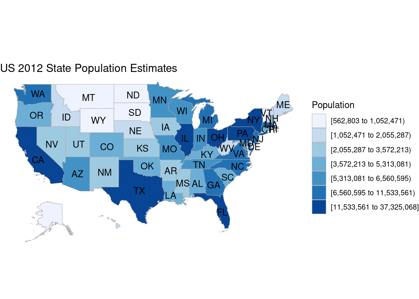
Choropleth maps
state_choropleth(df_pop_state,
                 title  = "US 2012 State Population Estimates",
                 legend = "Population")
Warning in private$zoom == "alaska" || private$zoom == "hawaii": 'length(x) = 51
> 1' in coercion to 'logical(1)'

Warning in private$zoom == "alaska" || private$zoom == "hawaii": 'length(x) = 51
> 1' in coercion to 'logical(1)'
Heatmap
data(df_state_demographics)
# head(df_state_demographics)

df_state_demographics <- df_state_demographics %>% arrange(total_population)

X <- data.matrix(df_state_demographics[,2:8])

row.names(X) <- df_state_demographics[,1]

head(X)
                     total_population percent_white percent_black percent_asian
wyoming                        570134            85             1             1
district of columbia           619371            35            49             3
vermont                        625904            94             1             1
north dakota                   689781            88             1             1
alaska                         720316            63             3             5
south dakota                   825198            84             1             1
                     percent_hispanic per_capita_income median_rent
wyoming                             9             28902         647
district of columbia               10             45290        1154
vermont                             2             29167         754
north dakota                        2             29732         564
alaska                              6             32651         978
south dakota                        3             25740         517
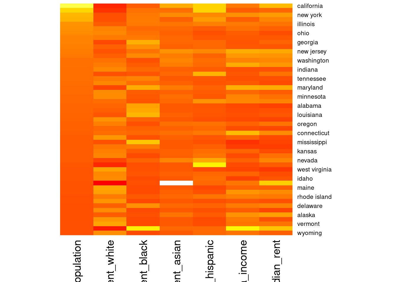
Heatmap using base R
heatmap(X, Rowv=NA, Colv=NA, col = cm.colors(256), scale = "column")
Heatmap using base R
heatmap(X, Rowv=NA, Colv=NA, col = heat.colors(256), scale = "column")
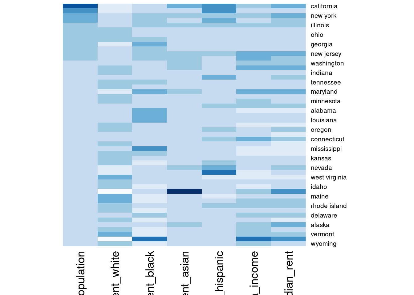
Heatmap using base R
library(RColorBrewer)

heatmap(X, Rowv=NA, Colv=NA, col = brewer.pal(9, "Blues"), scale = "column")
Heatmaply, using plotyly
library(plotly)
library(heatmaply)

heatmaply(X,scale = "col")
shinyHeatmaply, using plotyly
library(shinyHeatmaply)

launch_heatmaply(X)