---
title: "Deep Dream"
output:
html_notebook:
theme: cerulean
highlight: textmate
---
```{r setup, include=FALSE}
knitr::opts_chunk$set(warning = FALSE, message = FALSE)
```
***
This notebook contains the code samples found in Chapter 8, Section 2 of [Deep Learning with R](https://www.manning.com/books/deep-learning-with-r). Note that the original text features far more content, in particular further explanations and figures: in this notebook, you will only find source code and related comments.
***
## Implementing Deep Dream in Keras
We will start from a convnet pre-trained on ImageNet. In Keras, we have many such convnets available: VGG16, VGG19, Xception, ResNet50... albeit the same process is doable with any of these, your convnet of choice will naturally affect your visualizations, since different convnet architectures result in different learned features. The convnet used in the original Deep Dream release was an Inception model, and in practice Inception is known to produce very nice-looking Deep Dreams, so we will use the InceptionV3 model that comes with Keras.
```{r}
library(keras)
# We will not be training our model,
# so we use this command to disable all training-specific operations
k_set_learning_phase(0)
# Build the InceptionV3 network.
# The model will be loaded with pre-trained ImageNet weights.
model <- application_inception_v3(
weights = "imagenet",
include_top = FALSE,
)
```
Next, we compute the "loss", the quantity that we will seek to maximize during the gradient ascent process. In Chapter 5, for filter visualization, we were trying to maximize the value of a specific filter in a specific layer. Here we will simultaneously maximize the activation of all filters in a number of layers. Specifically, we will maximize a weighted sum of the L2 norm of the activations of a set of high-level layers. The exact set of layers we pick (as well as their contribution to the final loss) has a large influence on the visuals that we will be able to produce, so we want to make these parameters easily configurable. Lower layers result in geometric patterns, while higher layers result in visuals in which you can recognize some classes from ImageNet (e.g. birds or dogs). We'll start from a somewhat arbitrary configuration involving four layers -- but you will definitely want to explore many different configurations later on:
```{r}
# Named mapping layer names to a coefficient
# quantifying how much the layer's activation
# will contribute to the loss we will seek to maximize.
# Note that these are layer names as they appear
# in the built-in InceptionV3 application.
# You can list all layer names using `summary(model)`.
layer_contributions <- list(
mixed2 = 0.2,
mixed3 = 3,
mixed4 = 2,
mixed5 = 1.5
)
```
Now let's define a tensor that contains our loss, i.e. the weighted sum of the L2 norm of the activations of the layers listed above.
```{r}
# Get the symbolic outputs of each "key" layer (we gave them unique names).
layer_dict <- model$layers
names(layer_dict) <- lapply(layer_dict, function(layer) layer$name)
# Define the loss.
loss <- k_variable(0)
for (layer_name in names(layer_contributions)) {
# Add the L2 norm of the features of a layer to the loss.
coeff <- layer_contributions[[layer_name]]
activation <- layer_dict[[layer_name]]$output
scaling <- k_prod(k_cast(k_shape(activation), "float32"))
loss <- loss + (coeff * k_sum(k_square(activation)) / scaling)
}
```
Now we can set up the gradient ascent process:
```{r}
# This holds our generated image
dream <- model$input
# Normalize gradients.
grads <- k_gradients(loss, dream)[[1]]
grads <- grads / k_maximum(k_mean(k_abs(grads)), 1e-7)
# Set up function to retrieve the value
# of the loss and gradients given an input image.
outputs <- list(loss, grads)
fetch_loss_and_grads <- k_function(list(dream), outputs)
eval_loss_and_grads <- function(x) {
outs <- fetch_loss_and_grads(list(x))
loss_value <- outs[[1]]
grad_values <- outs[[2]]
list(loss_value, grad_values)
}
gradient_ascent <- function(x, iterations, step, max_loss = NULL) {
for (i in 1:iterations) {
c(loss_value, grad_values) %<-% eval_loss_and_grads(x)
if (!is.null(max_loss) && loss_value > max_loss)
break
cat("...Loss value at", i, ":", loss_value, "\n")
x <- x + (step * grad_values)
}
x
}
```
Finally, here is the actual Deep Dream algorithm.
First, we define a list of "scales" (also called "octaves") at which we will process the images. Each successive scale is larger than previous one by a factor 1.4 (i.e. 40% larger): we start by processing a small image and we increasingly upscale it:
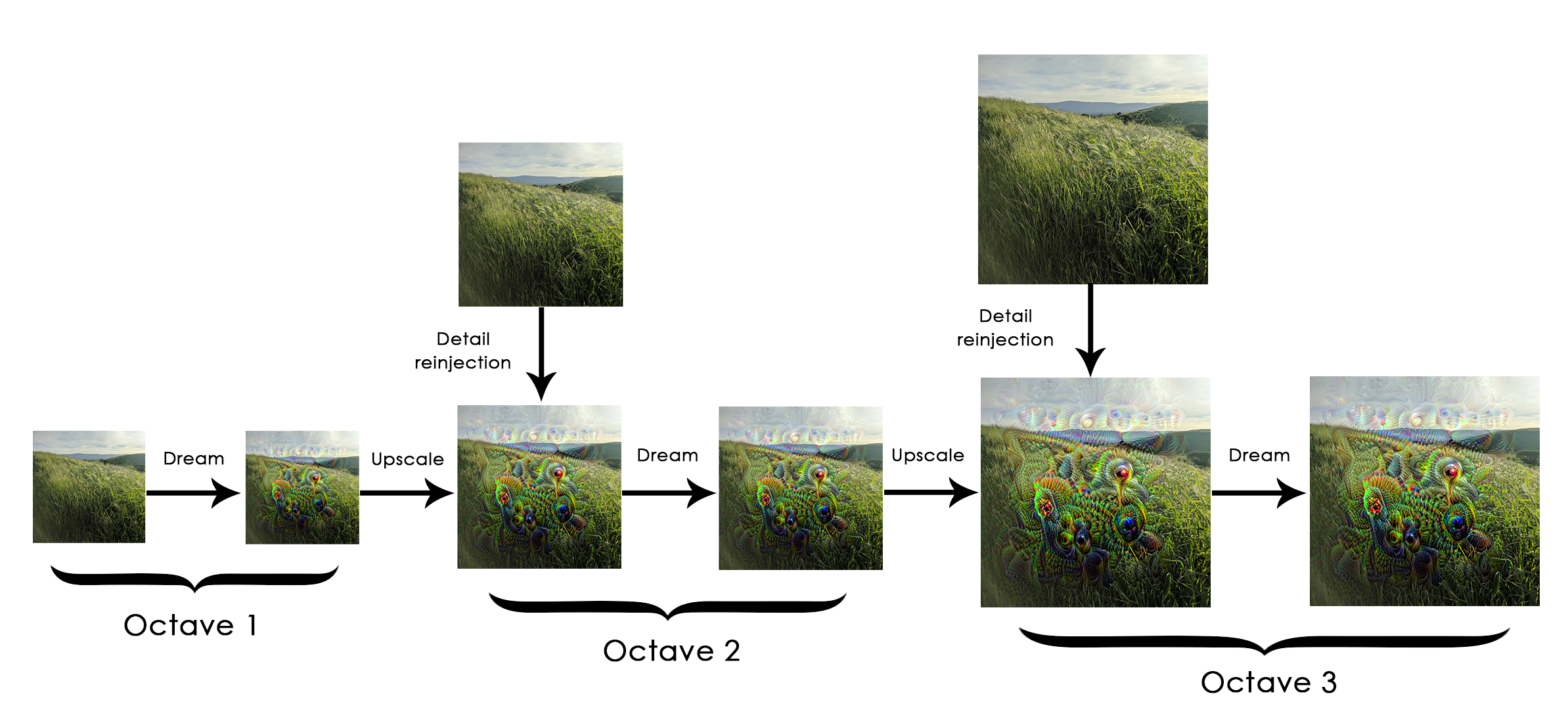
Then, for each successive scale, from the smallest to the largest, we run gradient ascent to maximize the loss we have previously defined, at that scale. After each gradient ascent run, we upscale the resulting image by 40%.
To avoid losing a lot of image detail after each successive upscaling (resulting in increasingly blurry or pixelated images), we leverage a simple trick: after each upscaling, we reinject the lost details back into the image, which is possible since we know what the original image should look like at the larger scale. Given a small image S and a larger image size L, we can compute the difference between the original image (assumed larger than L) resized to size L and the original resized to size S -- this difference quantifies the details lost when going from S to L.
```{r}
resize_img <- function(img, size) {
image_array_resize(img, size[[1]], size[[2]])
}
save_img <- function(img, fname) {
img <- deprocess_image(img)
image_array_save(img, fname)
}
# Util function to open, resize, and format pictures into appropriate tensors
preprocess_image <- function(image_path) {
image_load(image_path) %>%
image_to_array() %>%
array_reshape(dim = c(1, dim(.))) %>%
inception_v3_preprocess_input()
}
# Util function to convert a tensor into a valid image
deprocess_image <- function(img) {
img <- array_reshape(img, dim = c(dim(img)[[2]], dim(img)[[3]], 3))
img <- img / 2
img <- img + 0.5
img <- img * 255
dims <- dim(img)
img <- pmax(0, pmin(img, 255))
dim(img) <- dims
img
}
```
```{r}
# Playing with these hyperparameters will also allow you to achieve new effects
step <- 0.01 # Gradient ascent step size
num_octave <- 3 # Number of scales at which to run gradient ascent
octave_scale <- 1.4 # Size ratio between scales
iterations <- 20 # Number of ascent steps per scale
# If our loss gets larger than 10,
# we will interrupt the gradient ascent process, to avoid ugly artifacts
max_loss <- 10
# Fill this to the path to the image you want to use
dir.create("dream")
base_image_path <- "~/Downloads/African_Bush_Elephants.jpg"
# Load the image into an array
img <- preprocess_image(base_image_path)
# We prepare a list of shapes
# defining the different scales at which we will run gradient ascent
original_shape <- dim(img)[-1]
successive_shapes <- list(original_shape)
for (i in 1:num_octave) {
shape <- as.integer(original_shape / (octave_scale ^ i))
successive_shapes[[length(successive_shapes) + 1]] <- shape
}
# Reverse list of shapes, so that they are in increasing order
successive_shapes <- rev(successive_shapes)
# Resize the array of the image to our smallest scale
original_img <- img
shrunk_original_img <- resize_img(img, successive_shapes[[1]])
for (shape in successive_shapes) {
cat("Processsing image shape", shape, "\n")
img <- resize_img(img, shape)
img <- gradient_ascent(img,
iterations = iterations,
step = step,
max_loss = max_loss)
upscaled_shrunk_original_img <- resize_img(shrunk_original_img, shape)
same_size_original <- resize_img(original_img, shape)
lost_detail <- same_size_original - upscaled_shrunk_original_img
img <- img + lost_detail
shrunk_original_img <- resize_img(original_img, shape)
save_img(img, fname = sprintf("dream/at_scale_%s.png",
paste(shape, collapse = "x")))
}
save_img(img, fname = "dream/final_dream.png")
```
```{r}
plot(as.raster(deprocess_image(img) / 255))
```