|
CSU |
Hayward |
|
|
|
Statistics |
Department |
Appendix
B: A Very Brief Introduction
To Bayesian Inference
Prior Distributions and Expert Knowledge
The Bayesian approach to statistical inference treats population parameters as random variables. The distributions of these parameters are called prior distributions. Often both expert knowledge and mathematical convenience play a role in selecting a particular type of prior distribution.
|
For example, suppose that Proposition A is on the ballot for an upcoming statewide election, and that a political consultant has been hired to help manage the campaign for its passage. The proportion P of prospective voters who currently favor Prop. A is the population parameter of interest here. Based on her knowledge of the politics of the state, the consultant's judgment is that the proposition is almost sure to pass, but not by a large margin. She believes that the most likely proportion of voters in favor is 55% and that the percentage is not likely to be below 51% or above 59%. We use a beta distribution to model the expert's opinion. The beta family of distributions has density functions of the form f(p) = K1pa–1(1 – p)b–1, 0 < p < 1. where a, b > 0, and where K1 is a constant chosen so that f(p) integrates to 1 over (0, 1). A member of the beta family that corresponds roughly to the expert's opinion has a = 331 and b = 271.
Of course, many other distributional shapes share these two numerical properties, but we choose a member of the beta family because it makes the mathematics easier and because we have no reason to believe its shape is inappropriate here. |
Data and Posterior Distributions
The second step in Bayesian inference is to
collect data and to combine the information in the data with the expert opinion
represented by the prior distribution. The result is a posterior
distribution that can be used for inference. The computation of the
posterior distribution uses Bayes' Theorem. You have probably seen
Bayes' Theorem stated for an event E and a partition
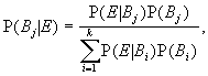
for
A more general version of Bayes' Theorem for distributions involving data x and a parameter p is as follows:
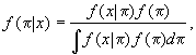
where the integral is taken over the region where the integrand is positive. The denominator of this fraction is a constant J. The conditional density f(p|x) is the posterior distribution of P given X, evaluated for the specific numerical values X = x and P = p.
|
In our election example, suppose n = 1000 subjects are selected at random. Assuming the specific parameter value P = p, the number X of them in favor of Prop. A is a random variable with the binomial distribution f(x|p) = K2 px(1 – p)n–x, for x = 0, 1, 2, ..., n, and where K2 = n!/[x!(n–x)!] is the constant that makes the distribution sum to 1. Then the general version of Bayes' Theorem gives the posterior distribution f(p|x) = K3px(1 – p)n–x pa–1(1 – p)b–1= K3px+a–1(1 – p)n–x+b–1, where K3 = K1K2/J. If x = 621 of the n = 1000 subjects interviewed favor Prop. A, it is then clear that the posterior has a beta distribution with parameters x + a = 952 and n – x + b = 650. According to this posterior distribution, P(0.570 < P < 0.618) = 0.95, so that a 95% posterior probability interval for the percent in favor is (57.0%, 61.8%). Note the following three aspects of this development:
|
Influence of Priors and Uninformative Priors
One factor of concern in Bayesian inference is how strongly the particular selection of a prior distribution influences the results of the inference. Particularly if results are to be used by people who may question the expert's opinion, it is desirable to have enough data that the influence of the prior is slight.
An uninformative prior (sometimes called a flat prior) is one that provides little or no information. Depending on the situation, uninformative priors may be quite disperse, may avoid only impossible or quite preposterous values of the parameter, or may not have modes. Uninformative priors sometimes give results similar to those obtained by traditional frequentist (i.e., non-Bayesian) methods.
|
Returning once again to our election example, suppose that another expert also believes that Prop. A is more likely than not to pass, but his views about current public opinion are more vague. Perhaps his beta prior has parameters 56 and 46. This prior also has mode 55%, but here P(0.45 < P < 0.64) = 0.95. Without seeing any data, he gives Prop. A a non-trivial chance of losing if the election were held today: P(P < 0.5) = 0.16. After he sees the results of the poll with 621 out of 1000 in favor, his posterior beta distribution has parameters 677 and 425, so that his 95% posterior interval estimate is (59.5%, 65.2%). The reasonable choice for an uninformative prior in this situation is the uniform distribution (which is beta with parameters 1 and 1, and which has no mode); it gives the 95% posterior interval estimate (59.1%, 65.1%). In this example, the 1000 observations are enough data that the two expert priors and the uninformative prior all give quite similar results. (The agreement would not be so good with a small amount of data.) A non-Bayesian 95% confidence interval, based on the normal approximation, is (59.1%. 65.1%). |
For a more extensive introduction to Bayesian inference see Hal S. Stern's article "A Primer on the Bayesian Approach to Statistical Inference" in STATS, 23 (Winter, 1998), pages 3-9.